MPC自动驾驶横向控制算法实现 c++-尧图网站建设

参考博客：
（1）无人车系统（十一）：轨迹跟踪模型预测控制(MPC)原理与python实现【40行代码】
（2）【自动驾驶】模型预测控制(MPC)实现轨迹跟踪
（3）自动驾驶——模型预测控制（MPC）理解与实践
（4）MPC算法学习(1)

0 前言

在这里插入图片描述
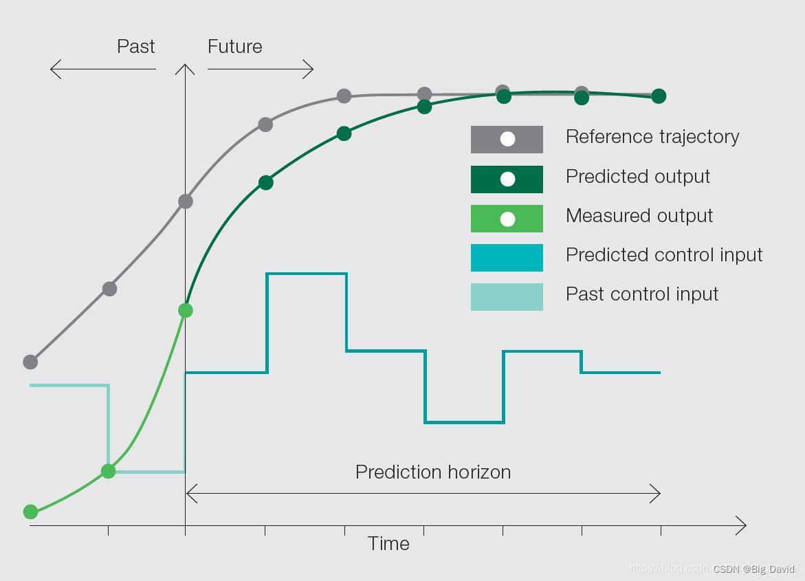
前面介绍的PID、Pure pursuit、Stanley都只是利用当前的系统误差来设计控制器。每个控制周期只选择一个目标路点作为跟踪对象，以上控制器只利用了模型进行向前一步预测。那么如果在更远的未来，参考轨迹变化不是那么平缓，并且有很多弯度小（急）的部分，那么只利用一步预测很难对整条轨迹进行有效的跟踪。

为了让无人车的控制器更有远见，设计控制器必须得利用模型对未来状态进行多步预测。由此引入MPC

1 模型预测控制原理

1.1 核心思想

MPC最核心的思想就是利用三维的空间模型加上时间构成四维时空模型，然后在这个时空模型的基础上，求解最优控制器。MPC基于一段时间的时空模型，得到的控制输出也是系统在未来有限时间步的控制序列。因为理论构建的模型与系统真实模型有误差；从而，更远未来的控制输出对系统控制的价值很低，MPC仅执行输出序列的第一个控制输出。
在这里插入图片描述

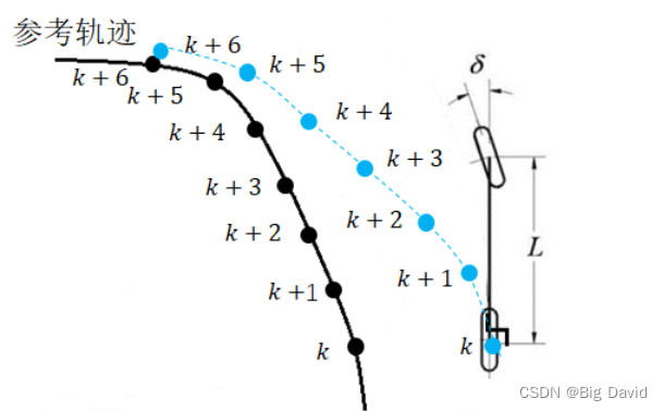
假设向前预测步长为 $T$ ，那么 $T$ 步的时空模型要比原始的空间模型大很多。MPC在每个控制周期都需要重新利用未来 $T$ 步的模型计算得到当前执行的控制指令。MPC利用了一个比原始空间模型大很多的模型仅仅只得到当前一步的最优控制器（和PID、Pure pursuit、Stanley做了同样的事）

MPC仅考虑未来几个时间步，一定程度上牺牲了最优性。

1.2 MPC优点

① 善于处理多输入多输出系统
② 可以处理约束，如安全性约束，上下阈值
③ MPC是一种向前考虑未来时间步的有限时域优化方法（一定的预测能力）
最优控制要求在整个时间优化，MPC采用了折中的策略，既不是像最优控制那样考虑整个时域，也不是仅仅考虑当前，而是考虑未来的有限时间域

1.3 MPC流程

模型预测控制在k时刻共有三步：
（1）获取系统当前的状态
（2）基于u(k)，u(k+1)，u(k+2)，…，u(k+m)进行最优化处理
离散系统的代价函数：
$J=\sum_{k}^{m-1} E^T_kQE_k+u^T_kRu_k+E^T_NFE_N$
$E_N$ 表示误差的终值，也是衡量优劣的标准
（3）只取u(k)作为控制输入施加在系统上

在下一时刻重复上面三步，在下一步进行预测时使用的就是下一步的状态值，我们将这样的方案称为滚动优化控制。

1.4 MPC vs LQR

	MPC	LQR
研究对象	线性和非线性系统均可	线性系统
状态方程：离散化	对非线性的状态方程进行线性化,对线性方程离散化	对线性方程离散化
目标函数	MPC目标函数一个是累计和	LQR目标函数一个是积分
求解方法	转化为二次规划问题，利用求解器进行求解，生成控制序列	采用变分法，通过求解黎卡提方程进行逼近，最终获取控制序列
工作时域	是求解预测时间段Np内的控制序列，并在下个周期后进行滚动优化	求解预测时间段内的控制序列，只求解一次，每个周期下取对应的控制量
LQR和MPC的优缺点	计算量大，实时性差，对于算力要求高，硬件成本较高	① LQR不滚动优化，预测时间段内的控制序列只求解一次，没有考虑实际与规划的误差② LQR求解整个预测时域内的控制序列，而MPC可在更小的时间窗口中求解优化问题，获得次优解，可大大提升求解速度③ 无约束，假设对控制量无约束

2 MPC控制器设计

2.1 线性模型

当模型是线性的，MPC求解可以转化为一个二次规划问题。
线性模型： $x_{k+1}=Ax_k+Bu_k+C$
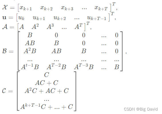
假定未来T步的控制输入已知，为 $u_k,u_{k+1},u_{k+2},...,u_{k+T}$ ，根据以上模型与输入，可以计算未来 T 步的状态：
在这里插入图片描述
矩阵向量形式： $X=Ax _k +B_u+C$
其中，

2.2 非线性模型

线性化过程损失了模型精度。
无人车几何运动学模型：
在这里插入图片描述
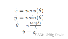
将以上连续的微分模型离散化成差分模型(差分间隔为 $d_t$ )：

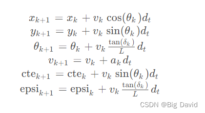
假定无人车需要跟踪的轨迹由离散点{ $(\bar{x}_1,\bar{y}_1),(\bar{x}_2,\bar{y}_2),...,(\bar{x}_M,\bar{y}_M)$ }通过三次曲线拟合而成，可表示成由x轴为自变量的函数： $y=f(x)=c_0x^3+c_1x^2+c_2x+c_3$ 。

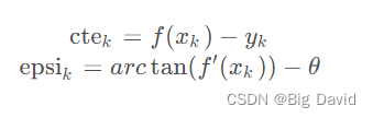
在每一个预测步，可以根据无人车的 $x_k$ 与 $y_k$ 值计算横向跟踪误差 $cte_k$ 与航向偏差 $epsi_k$ 。
在这里插入图片描述

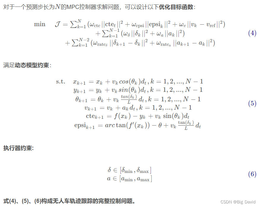
2.3 约束

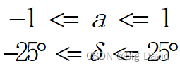
对于约束，一般分为Hard约束和Soft约束。Hard约束是不可违背必须遵守的，在控制系统中，输入输出都可能会有约束限制，但是在设计时不建议将输入输出都给予Hard约束，因为这两个约束有可能会有重叠，导致优化器会产生不可行解。

建议输出采用Soft约束，而输入的话建议输入和输入参数变化率二者之间不要同时为Hard约束，可以一个Hard一个Soft。

3 MPC - 无人车轨迹跟踪

车辆的状态量偏差和控制量偏差：
$\tilde{\boldsymbol{x}}=\left[\begin{array}{c} \dot{x}-\dot{x}_{r} \\ \dot{y}-\dot{y}_{r} \\ \dot{\varphi}-\dot{\varphi}_{r} \end{array}\right], \tilde{\boldsymbol{u}}=\left[\begin{array}{c} v-v_{r} \\ \delta-\delta_{r} \end{array}\right]$

PID控制器轨迹跟随实现博客里的运动学模型的离散状态空间方程：
$\tilde{\boldsymbol{x}}(k+1)=\left[\begin{array}{ccc} 1 & 0 & -T v_{r} \sin \varphi_{r} \\ 0 & 1 & T v_{r} \cos \varphi_{r} \\ 0 & 0 & 1 \end{array}\right] \tilde{\boldsymbol{x}}(k)+\left[\begin{array}{cc} T \cos \varphi_{r} & 0 \\ T \sin \varphi_{r} & 0 \\ T \frac{\tan \delta_{r}}{l} & T \frac{v_{r}}{l \cos ^{2} \delta_{r}} \end{array}\right] \tilde{\boldsymbol{u}}(k)$

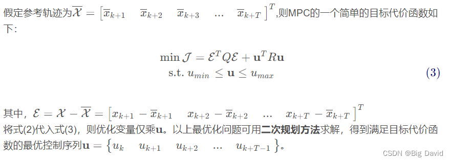
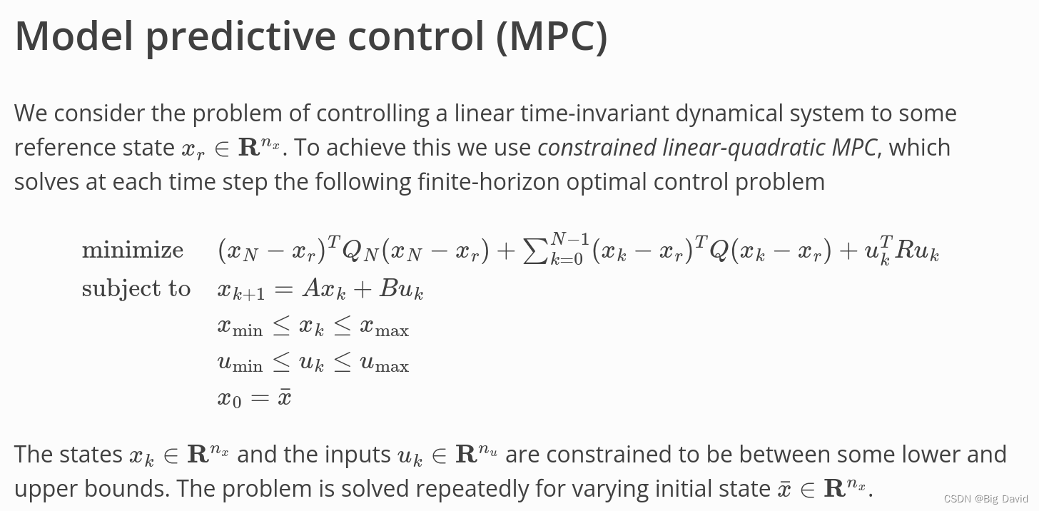
为了表示控制系统达到稳定控制所付出的代价，MPC控制的代价函数：
$\min J(\boldsymbol{U})=\sum_{k=0}^{N-1}\left(\tilde{\boldsymbol{x}}(k)^{T} Q \tilde{\boldsymbol{x}}(k)+\tilde{\boldsymbol{u}}(k)^{T} R \tilde{\boldsymbol{u}}(k)\right)+\tilde{\boldsymbol{x}}(N)^{T} Q_{f} \tilde{\boldsymbol{x}}(N)$

其中，
$U=(u_0,u_1,...,u_N)$ ，并且矩阵 $Q,Q_f,R$ 为正定矩阵
$Q$ ：给定状态代价矩阵
$Q_f$ ：最终状态代价矩阵
$R$ ：输入代价矩阵
$N$ ：时间范围
$R > 0$ ：任何非0输入都增加 $J$ 的代价

对于 $\min J(\boldsymbol{U})=\sum_{k=0}^{N-1}\left(\tilde{\boldsymbol{x}}(k)^{T} Q \tilde{\boldsymbol{x}}(k)+\tilde{\boldsymbol{u}}(k)^{T} R \tilde{\boldsymbol{u}}(k)\right)+\tilde{\boldsymbol{x}}(N)^{T} Q_{f} \tilde{\boldsymbol{x}}(N)$ ，需要服从的约束条件包括：
① 运动学模型约束 —— $\tilde{\boldsymbol{x}}(k+1)=\boldsymbol{A} \tilde{\boldsymbol{x}}(k)+\boldsymbol{B} \tilde{\boldsymbol{u}}(k)$
② 控制量约束 —— $|\tilde{\boldsymbol{u}}(k)| \leq \tilde{\boldsymbol{u}}_{\max }$
③ 初始状态 —— $\tilde{\boldsymbol{x}}(0)=\tilde{\boldsymbol{x}}_{0}$

osqp-eigen官网给出的MPC例子
MPCExample.cpp
在这里插入图片描述

// osqp-eigen
#include "OsqpEigen/OsqpEigen.h"// eigen
#include <Eigen/Dense>#include <iostream>void setDynamicsMatrices(Eigen::Matrix<double, 12, 12>& a, Eigen::Matrix<double, 12, 4>& b)
{a << 1., 0., 0., 0., 0., 0., 0.1, 0., 0., 0., 0., 0., 0., 1., 0., 0., 0., 0., 0., 0.1, 0., 0.,0., 0., 0., 0., 1., 0., 0., 0., 0., 0., 0.1, 0., 0., 0., 0.0488, 0., 0., 1., 0., 0., 0.0016,0., 0., 0.0992, 0., 0., 0., -0.0488, 0., 0., 1., 0., 0., -0.0016, 0., 0., 0.0992, 0., 0.,0., 0., 0., 0., 1., 0., 0., 0., 0., 0., 0.0992, 0., 0., 0., 0., 0., 0., 1., 0., 0., 0., 0.,0., 0., 0., 0., 0., 0., 0., 0., 1., 0., 0., 0., 0., 0., 0., 0., 0., 0., 0., 0., 0., 1., 0.,0., 0., 0.9734, 0., 0., 0., 0., 0., 0.0488, 0., 0., 0.9846, 0., 0., 0., -0.9734, 0., 0., 0.,0., 0., -0.0488, 0., 0., 0.9846, 0., 0., 0., 0., 0., 0., 0., 0., 0., 0., 0., 0., 0.9846;b << 0., -0.0726, 0., 0.0726, -0.0726, 0., 0.0726, 0., -0.0152, 0.0152, -0.0152, 0.0152, -0.,-0.0006, -0., 0.0006, 0.0006, 0., -0.0006, 0.0000, 0.0106, 0.0106, 0.0106, 0.0106, 0,-1.4512, 0., 1.4512, -1.4512, 0., 1.4512, 0., -0.3049, 0.3049, -0.3049, 0.3049, -0.,-0.0236, 0., 0.0236, 0.0236, 0., -0.0236, 0., 0.2107, 0.2107, 0.2107, 0.2107;
}void setInequalityConstraints(Eigen::Matrix<double, 12, 1>& xMax,Eigen::Matrix<double, 12, 1>& xMin,Eigen::Matrix<double, 4, 1>& uMax,Eigen::Matrix<double, 4, 1>& uMin)
{double u0 = 10.5916;// input inequality constraintsuMin << 9.6 - u0, 9.6 - u0, 9.6 - u0, 9.6 - u0;uMax << 13 - u0, 13 - u0, 13 - u0, 13 - u0;// state inequality constraintsxMin << -M_PI / 6, -M_PI / 6, -OsqpEigen::INFTY, -OsqpEigen::INFTY, -OsqpEigen::INFTY, -1.,-OsqpEigen::INFTY, -OsqpEigen::INFTY, -OsqpEigen::INFTY, -OsqpEigen::INFTY,-OsqpEigen::INFTY, -OsqpEigen::INFTY;xMax << M_PI / 6, M_PI / 6, OsqpEigen::INFTY, OsqpEigen::INFTY, OsqpEigen::INFTY,OsqpEigen::INFTY, OsqpEigen::INFTY, OsqpEigen::INFTY, OsqpEigen::INFTY, OsqpEigen::INFTY,OsqpEigen::INFTY, OsqpEigen::INFTY;
}void setWeightMatrices(Eigen::DiagonalMatrix<double, 12>& Q, Eigen::DiagonalMatrix<double, 4>& R)
{Q.diagonal() << 0, 0, 10., 10., 10., 10., 0, 0, 0, 5., 5., 5.;R.diagonal() << 0.1, 0.1, 0.1, 0.1;
}void castMPCToQPHessian(const Eigen::DiagonalMatrix<double, 12>& Q,const Eigen::DiagonalMatrix<double, 4>& R,int mpcWindow,Eigen::SparseMatrix<double>& hessianMatrix)
{hessianMatrix.resize(12 * (mpcWindow + 1) + 4 * mpcWindow,12 * (mpcWindow + 1) + 4 * mpcWindow);// populate hessian matrixfor (int i = 0; i < 12 * (mpcWindow + 1) + 4 * mpcWindow; i++){if (i < 12 * (mpcWindow + 1)){int posQ = i % 12;float value = Q.diagonal()[posQ];if (value != 0)hessianMatrix.insert(i, i) = value;} else{int posR = i % 4;float value = R.diagonal()[posR];if (value != 0)hessianMatrix.insert(i, i) = value;}}
}void castMPCToQPGradient(const Eigen::DiagonalMatrix<double, 12>& Q,const Eigen::Matrix<double, 12, 1>& xRef,int mpcWindow,Eigen::VectorXd& gradient)
{Eigen::Matrix<double, 12, 1> Qx_ref;Qx_ref = Q * (-xRef);// populate the gradient vectorgradient = Eigen::VectorXd::Zero(12 * (mpcWindow + 1) + 4 * mpcWindow, 1);for (int i = 0; i < 12 * (mpcWindow + 1); i++){int posQ = i % 12;float value = Qx_ref(posQ, 0);gradient(i, 0) = value;}
}void castMPCToQPConstraintMatrix(const Eigen::Matrix<double, 12, 12>& dynamicMatrix,const Eigen::Matrix<double, 12, 4>& controlMatrix,int mpcWindow,Eigen::SparseMatrix<double>& constraintMatrix)
{constraintMatrix.resize(12 * (mpcWindow + 1) + 12 * (mpcWindow + 1) + 4 * mpcWindow,12 * (mpcWindow + 1) + 4 * mpcWindow);// populate linear constraint matrixfor (int i = 0; i < 12 * (mpcWindow + 1); i++){constraintMatrix.insert(i, i) = -1;}for (int i = 0; i < mpcWindow; i++)for (int j = 0; j < 12; j++)for (int k = 0; k < 12; k++){float value = dynamicMatrix(j, k);if (value != 0){constraintMatrix.insert(12 * (i + 1) + j, 12 * i + k) = value;}}for (int i = 0; i < mpcWindow; i++)for (int j = 0; j < 12; j++)for (int k = 0; k < 4; k++){float value = controlMatrix(j, k);if (value != 0){constraintMatrix.insert(12 * (i + 1) + j, 4 * i + k + 12 * (mpcWindow + 1))= value;}}for (int i = 0; i < 12 * (mpcWindow + 1) + 4 * mpcWindow; i++){constraintMatrix.insert(i + (mpcWindow + 1) * 12, i) = 1;}
}void castMPCToQPConstraintVectors(const Eigen::Matrix<double, 12, 1>& xMax,const Eigen::Matrix<double, 12, 1>& xMin,const Eigen::Matrix<double, 4, 1>& uMax,const Eigen::Matrix<double, 4, 1>& uMin,const Eigen::Matrix<double, 12, 1>& x0,int mpcWindow,Eigen::VectorXd& lowerBound,Eigen::VectorXd& upperBound)
{// evaluate the lower and the upper inequality vectorsEigen::VectorXd lowerInequality= Eigen::MatrixXd::Zero(12 * (mpcWindow + 1) + 4 * mpcWindow, 1);Eigen::VectorXd upperInequality= Eigen::MatrixXd::Zero(12 * (mpcWindow + 1) + 4 * mpcWindow, 1);for (int i = 0; i < mpcWindow + 1; i++){lowerInequality.block(12 * i, 0, 12, 1) = xMin;upperInequality.block(12 * i, 0, 12, 1) = xMax;}for (int i = 0; i < mpcWindow; i++){lowerInequality.block(4 * i + 12 * (mpcWindow + 1), 0, 4, 1) = uMin;upperInequality.block(4 * i + 12 * (mpcWindow + 1), 0, 4, 1) = uMax;}// evaluate the lower and the upper equality vectorsEigen::VectorXd lowerEquality = Eigen::MatrixXd::Zero(12 * (mpcWindow + 1), 1);Eigen::VectorXd upperEquality;lowerEquality.block(0, 0, 12, 1) = -x0;upperEquality = lowerEquality;lowerEquality = lowerEquality;// merge inequality and equality vectorslowerBound = Eigen::MatrixXd::Zero(2 * 12 * (mpcWindow + 1) + 4 * mpcWindow, 1);lowerBound << lowerEquality, lowerInequality;upperBound = Eigen::MatrixXd::Zero(2 * 12 * (mpcWindow + 1) + 4 * mpcWindow, 1);upperBound << upperEquality, upperInequality;
}void updateConstraintVectors(const Eigen::Matrix<double, 12, 1>& x0,Eigen::VectorXd& lowerBound,Eigen::VectorXd& upperBound)
{lowerBound.block(0, 0, 12, 1) = -x0;upperBound.block(0, 0, 12, 1) = -x0;
}double getErrorNorm(const Eigen::Matrix<double, 12, 1>& x, const Eigen::Matrix<double, 12, 1>& xRef)
{// evaluate the errorEigen::Matrix<double, 12, 1> error = x - xRef;// return the normreturn error.norm();
}int main()
{// set the preview windowint mpcWindow = 20;// allocate the dynamics matricesEigen::Matrix<double, 12, 12> a;Eigen::Matrix<double, 12, 4> b;// allocate the constraints vectorEigen::Matrix<double, 12, 1> xMax;Eigen::Matrix<double, 12, 1> xMin;Eigen::Matrix<double, 4, 1> uMax;Eigen::Matrix<double, 4, 1> uMin;// allocate the weight matricesEigen::DiagonalMatrix<double, 12> Q;Eigen::DiagonalMatrix<double, 4> R;// allocate the initial and the reference state spaceEigen::Matrix<double, 12, 1> x0;Eigen::Matrix<double, 12, 1> xRef;// allocate QP problem matrices and vectoresEigen::SparseMatrix<double> hessian;Eigen::VectorXd gradient;Eigen::SparseMatrix<double> linearMatrix;Eigen::VectorXd lowerBound;Eigen::VectorXd upperBound;// set the initial and the desired statesx0 << 0, 0, 0, 0, 0, 0, 0, 0, 0, 0, 0, 0;xRef << 0, 0, 1, 0, 0, 0, 0, 0, 0, 0, 0, 0;// set MPC problem quantitiessetDynamicsMatrices(a, b);setInequalityConstraints(xMax, xMin, uMax, uMin);setWeightMatrices(Q, R);// cast the MPC problem as QP problemcastMPCToQPHessian(Q, R, mpcWindow, hessian);castMPCToQPGradient(Q, xRef, mpcWindow, gradient);castMPCToQPConstraintMatrix(a, b, mpcWindow, linearMatrix);castMPCToQPConstraintVectors(xMax, xMin, uMax, uMin, x0, mpcWindow, lowerBound, upperBound);// instantiate the solverOsqpEigen::Solver solver;// settings// solver.settings()->setVerbosity(false);solver.settings()->setWarmStart(true);// set the initial data of the QP solversolver.data()->setNumberOfVariables(12 * (mpcWindow + 1) + 4 * mpcWindow);solver.data()->setNumberOfConstraints(2 * 12 * (mpcWindow + 1) + 4 * mpcWindow);if (!solver.data()->setHessianMatrix(hessian))return 1;if (!solver.data()->setGradient(gradient))return 1;if (!solver.data()->setLinearConstraintsMatrix(linearMatrix))return 1;if (!solver.data()->setLowerBound(lowerBound))return 1;if (!solver.data()->setUpperBound(upperBound))return 1;// instantiate the solverif (!solver.initSolver())return 1;// controller input and QPSolution vectorEigen::Vector4d ctr;Eigen::VectorXd QPSolution;// number of iteration stepsint numberOfSteps = 50;for (int i = 0; i < numberOfSteps; i++){// solve the QP problemif (!solver.solve())return 1;// get the controller inputQPSolution = solver.getSolution();ctr = QPSolution.block(12 * (mpcWindow + 1), 0, 4, 1);// save data into fileauto x0Data = x0.data();// propagate the modelx0 = a * x0 + b * ctr;// update the constraint boundupdateConstraintVectors(x0, lowerBound, upperBound);if (!solver.updateBounds(lowerBound, upperBound))return 1;}return 0;
}

MPC.h

#pragma once#include <iostream>
#include <vector>
#include <Eigen/Dense>
#include "KinematicModel.h"
#include "OsqpEigen/OsqpEigen.h"
#include <osqp/osqp.h>
#include "matplotlibcpp.h"namespace plt = matplotlibcpp;
using namespace std;
using namespace Eigen;
using namespace OsqpEigen;namespace {const double MAX_STEER = M_PI / 6.0;const double MAX_VEL = 10.0;
}
class MPC {
private:int NX, NU, T;MatrixXd R = MatrixXd::Identity(NU, NU);MatrixXd Rd = MatrixXd::Identity(NU, NU);MatrixXd Q = MatrixXd::Identity(NX, NX);MatrixXd Qf = Q;
public:MPC(int nx, int nu, int t);vector<double> LMPC(MatrixXd xref, Vector3d x0, MatrixXd ref_delta, KinematicModel model);
};

MPC.cpp

#include "MPC.h"MPC::MPC(int nx, int nu, int t) : NX(nx), NU(nu), T(t) {}vector<double> MPC::LMPC(MatrixXd xref, Vector3d x0, MatrixXd ref_delta, KinematicModel model)
{int NX = xref.rows();      // 3int NU = ref_delta.rows(); // 2int T = xref.cols() - 1;  // Horizon length. // 2// Define optimization variables.MatrixXd x(NX, T + 1); // 3, 3MatrixXd u(NU, T); // 1, 2// Store A matrices.vector<MatrixXd> A_vec;// Store B matrices.vector<MatrixXd> B_vec;// Initialize A and B matrices.for (int t = 0; t < T; ++t) {auto state_space = model.stateSpace(ref_delta(1, t), xref(2, t));A_vec.push_back(state_space[0]);B_vec.push_back(state_space[1]);}// Define the optimization problem.VectorXd cost(T + 1); // t + 1// List of constraint indices.vector<vector<int>> constraints;for (int t = 0; t < T; ++t) {cost(t) = (u.col(t) - ref_delta.col(t)).transpose() * R * (u.col(t) - ref_delta.col(t));if (t != 0) {cost(t) += (x.col(t) - xref.col(t)).transpose() * Q * (x.col(t) - xref.col(t));}MatrixXd A = A_vec[t];MatrixXd B = B_vec[t];// 3 6  6 9constraints.push_back({(t + 1) * NX, (t + 1) * NX + NX});  // State constraints.// 0 2 2 4constraints.push_back({t * NU, t * NU + NU});  // Input constraints.x.col(t + 1) = A * x.col(t) + B * (u.col(t) - ref_delta.col(t));}// Final state cost.cost(T) = (x.col(T) - xref.col(T)).transpose() * Qf * (x.col(T) - xref.col(T));// Set initial state.x.col(0) = x0; // 3VectorXd lower_bound(T * NU); // 4VectorXd upper_bound(T * NU); // 4for (int t = 0; t < T; t++){lower_bound.segment(t * NU, NU) << -MAX_VEL, -MAX_STEER; // (1:2) (3:4)upper_bound.segment(t * NU, NU) << MAX_VEL, MAX_STEER; // (1:2) (3:4)}// Solve the optimization problem.OsqpEigen::Solver solver;// solver.settings()->setVerbosity(false);solver.settings()->setWarmStart(true);// A: T * (NU + NX) x NX * (T + 1)// solver.data()->setNumberOfVariables(NX * (T + 1)); // 9// solver.data()->setNumberOfConstraints(T * (NU + NX));// 10solver.data()->setNumberOfVariables(NX * (T + 1)); //变量数n 9solver.data()->setNumberOfConstraints(T * (NU + NX));// 约束数m 10// P:NX * (T + 1) x NX * (T + 1)// Define the Hessian matrix dimension.int N = NX * (T + 1); // 9// Define and set the Hessian matrix.Eigen::SparseMatrix<double> P(N, N); // 9 x 9for (int t = 0; t < T; ++t) {for (int i = 0; i < NU; ++i) {P.coeffRef(t * NU + i, t * NU + i) = R(i, i);}}if (!solver.data()->setHessianMatrix(P)) return {};// Define the gradient vector (cost vector).VectorXd q(N); // 9 x 1for (int t = 0; t < T; ++t) {q.segment(t * NU, NU) = cost(t) * VectorXd::Ones(NU);}if (!solver.data()->setGradient(q)) return {};// Define the linear equality constraint matrix Aeq.int M = T * (NX + NU);  // Number of equality constraints. // M = 10Eigen::SparseMatrix<double> linearMatrix(M, N);  // 10 x 9for (int i = 0; i < M; i++){for (int j = 0; j < N; j++){if (i == j) linearMatrix.insert(i, j) = 1;else linearMatrix.insert(i, j) = 0;}}if (!solver.data()->setLinearConstraintsMatrix(linearMatrix)) return {};// Define the equality constraint vector beq.VectorXd beq(M); // 10 x 1//  for (int i = 0; i < M; i++)//  {//       beq(i) = 0;//   }// You should populate Aeq and beq based on your state dynamics.// Set lower and upper bounds for variables and constraints.if (!solver.data()->setLowerBound(lower_bound)) {cerr << "Error setting lower bound." << endl;return {};}if (!solver.data()->setUpperBound(upper_bound)) {cerr << "Error setting upper bound." << endl;return {};}// Initialize the solver.if (!solver.initSolver()) return {};// Solve the problem.if (!solver.solve()) {cerr << "Error solving the optimization problem." << endl;return {};}VectorXd optimal_solution = solver.getSolution();// Extract optimal control inputs.vector<double> optimal_input;for (int t = 0; t < T; ++t) {VectorXd u_t = optimal_solution.segment(t * NU, NU); // (1,2) (3,4)optimal_input.push_back(u_t(0));  // Extract the velocity input.}cout << optimal_input[1] << endl;return optimal_input;
}

main.cpp

#include "MPC.h"
#include "Reference_path.h"
#include "KinematicModel.h"
#include "matplotlibcpp.h"
#include "pid_controller.h"namespace plt = matplotlibcpp;int main()
{parameters param;param.NX = 3;param.NU = 2;param.T = 2;param.L = 2.2;param.dt = 0.1;double Target_speed = 8.0 / 3.6;MPC mpc(param.NX, param.NU, param.T);Eigen::VectorXd x0(param.NX);x0 << 0.0, -3.0, 0.0; // x y yawvector<double> robot_state = {0.0, -3.0, 0.0, 0.0};double dt = 0.1;double L = 2.2;ReferencePath reference_path;auto reference_trajectory = reference_path.calc_ref_trajectory(robot_state, param, 1.0);KinematicModel model(x0(0), x0(1), x0(2), 0.0, L, dt);PID_controller PID(3, 0.001, 30, Target_speed, 15.0 / 3.6, 0.0);std::vector<double> x_;std::vector<double> y_;for (int i = 0; i < param.T; i++){Eigen::MatrixXd xref = reference_trajectory.xref;Eigen::VectorXd xref_i = xref.col(i); // 3 x 1Eigen::VectorXd ref_delta = reference_trajectory.dref.col(i); // 2 x 1std::vector<double> control_input = mpc.LMPC(xref_i, x0, ref_delta, model);cout << control_input[1] << endl;double a = PID.calOutput(model.v);model.updateState(a, control_input[1]);cout << "Speed: " << model.v << " m/s" << endl;x_.push_back(model.getState()[0]);y_.push_back(model.getState()[1]);const auto state = model.getState();x0 << state[0], state[1], state[2];//画参考轨迹plt::plot(reference_path.ref_x, reference_path.ref_y, "b--");plt::grid(true);plt::ylim(-5, 5);plt::plot(x_, y_, "r");plt::pause(0.01);}const char* filename = "./MPC.png";plt::save(filename);plt::show();return 0;
}

MPC.cpp有bug，有空时更正

资讯详情

MPC自动驾驶横向控制算法实现 c++